The
Educational Achievement of Indian Children
CHAPTER III
Statistical Treatment
of the Test Data
INTRODUCTION
In order to make the report more meaningful to the
reader, it was decided to describe the statistical treatment of
the test data
in some detail. The discussion and interpretation of the results
depend directly upon this treatment. Then too, because of the great
amount of data gathered, certain assumptions had to be made in
order to facilitate the treatment of the data and the discussion
of the results. An understanding of these assumptions is necessary
to interpret and qualify the results properly.
GENERAL PROCEDURES
The test scores for each test for each student were entered on
a code sheet, transferred to Hollerith cards, and sorted by IBM
equipment. Since there were nine geographic areas and six types
of schools and twenty-four tests, the sorting yielded 360 distributions.
The following distribution for grade eight for day schools for
the Pressey Vocabulary Test was typical:
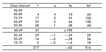
The following values were calculated for each of the 360 distributions:
(1) mean, (2) standard deviation, (3) plus one standard deviation,
and (4) minus one standard deviation. For the distribution shown
above, the calculations were as follows:
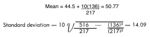
Plus one standard deviation = 50.77 + 14.09 = 64.86
Minus one standard
deviation = 50.77 - 14.09 = 36.68
These values were used to draw the vertical lines that appear on
the twenty-four figures in Chapter IV. There are nine of these
lines for the nine geographic
areas and six of these lines for the six types of schools.
These values were also used in computing the percentage of overlap between grade
eight and grade twelve for the various types of schools where the tests given
were common to both grade levels. For example, what percentage of the students
in the mission schools in grade eight exceeded the mean of the students in the
mission schools in grade twelve on the Use of Resources Test? The mean of the
pupils in grade twelve was 47.45 and the mean for the pupils in the eighth grade
was 37.91. The standard deviation for the eighth grade was 8.40. In terms of
the eighth grade distribution, how many standard deviations above the mean would
a score of 47.45 fall? The procedure is as follows:

Assuming a normal distribution of test scores for grade eight, 1.14 standard
deviations above the mean would have 12.7 per cent of the area above this point.
Therefore, it can be said, assuming a normal distribution of scores, that 12.7
per cent of the eighth grade exceeded the mean score of the twelfth grade on
the Use of Resources Test.
FURTHER ANALYSIS
Did the Indian children located in a particular geographic area achieve significantly
more on a particular test than the Indian children in the other eight areas?
In order to answer this question for the twenty-four tests, it would have been
necessary to run twenty-four tests of significance by means of the technique
of analysis of variance. Since this technique is based on the assumption of nomogeneity
of variances, this would have necessitated twenty-four tests for homogeneity
of variances prior to the application of the F test or test of significance.
If on a particular test, the geographic areas had been homogeneous with respect
to variances and if the F test had proved to be significant, thirty-six t tests
would have had to be run in order to locate the significant differences between
particular geographic areas. The required probability for the selected difference
to be significant would be 1.39 in 1000 at the 5 per cent level or the critical
ratio would have to be equal to or greater than about 3.22. Even a spot check
here and there would, at best, be sketchy because the number of cases in each
area varies considerably. Thus, in two different comparisons the one critical
ratio might be significant because of the large N's involved and the other critical
ratio might not be significant because of the small N's involved, even though
the differences in means were the some or nearly so. Needless to say, these calculations
would have involved an immense amount of labor. Therefore, any conclusions regarding
differences in achievement between geographic areas on the various tests, will
have to be drawn from the line graphs appearing in the various figures.
A word of explanation regarding the line graphs is in order. The distribution
for a particular test for a particular area or type of school is graphically
portrayed by a straight vertical line, the lowest point of the line being one
standard deviation below the mean (a horizontal mark at the center of the vertical
line), and the highest point of the line being one standard deviation above the
mean. These limits, assuming a normal distribution of scores, mark the range
of the middle two-thirds of the students on a particular test. The achievement
of Indian children in the various geographic areas or in the various types of
schools can be compared by locating the mean point. In addition, the amount of
overlap in achievement on a particular test can be noted by comparing the two
vertical lines for two geographic areas or for two types of schools.
These vertical lines were also drawn for the five types of schools which Indian
children attend. These five types of schools are: reservation boarding schools,
day schools, mission schools, non-reservation boarding schools, and public schools.*Since the Indian Service is more interested in the achievement of Indian children
in the various schools Indian children attend than in the comparison between
these types of schools and the schools which white children attend, it was decided
to go beyond the graphical treatment for these comparisons even though the amount
of labor involved was great.
Since the results of the IBM work yielded distributions of scores rather than
the sums of the scores and the sums of the scores squared, it would have been
awkward to use the technique of analysis of variance mentioned previously. An
examination of the line graphs made it almost certain that significant differences
based on comparisons between types of schools would have been obtained for all
twenty-four of the tests. Later calculations proved this examination to be correct.
For the moment, let us assume that F values had been calculated and that all
of the values were significant. Ordinarily one would not calculate the F values
unless the test of homogeneity of variances had established that the variabilities
of the groups under comparison were essentially the same. Were the variabilities
for the six types of schools on the twenty-four tests essentially the same or
did they differ significantly from each other? An examination of the data indicated
that on some of the tests, the six types of schools were homogeneous with respect
to variances and on other tests they were not. What effect would a significant
difference in variances have on the value obtained by running a t test on the
scores obtained from the two types of schools? It may result in a somewhat larger
value of t, but it is unlikely that a significant value of t would be produced
only by a difference in variances16 Since the data yielded by the IBM work lent
themselves better to the calculation of critical ratios rather than t ratios,
fifteen critical ratios were calculated for each of the twenty-four tests. A
comparison was made of the values yielded by the critical ratio formula with
those yielded by the t formula or by the use of the BehrensFisher formula when
the variances were not homogeneous.
In the case of the Pressey Vocabulary Test for grade eight, did the Indian children
in the public schools achieve significantly more than the Indian children in
the day schools? A critical ratio of 5.81 was obtained in favor of the Indian
children in the public schools. On the face of it, this would seem to indicate
that Indian children in the public schools achieved significantly more than did
the Indian children in the day schools. The application of the t test yielded
a value of 5.86, slightly higher than that obtained by the critical ratio formula.
However, the variances of the two groups were not homogeneous and the t test
was not the proper tool to use. The application of the Behrens-Fisher d test
yielded a value of 5.86 which exceeded the table value at the 1 per cent level.
This definitely established the superiority of the Indian children in the public
schools.
Although the procedure used with the comparison of achievement of Indian children
in public and day schools is correct where the variances differ significantly,
this procedure involves a great amount of unnecessary work, since the values
obtained by all three methods will not differ greatly when the number of cases
involved is large. Edwards has this to say: "With still larger samples,
in the neighborhood of 30 cases each, a variance which is 2.0 times as large
as the other will be sufficient to reject the hypothesis of a common variance."17
Since the number of cases in grade eight ranged from about 70 to 450 and since
the number of cases in grade twelve ranged from about 30 to 350, the consideration
of homogeneity of variances for this study did not seem to be important providing
the reader is mindful that significant differences in variances did exist in
a minority of the comparisons. Therefore, to facilitate the drawing of conclusions,
it was assumed that each of the twenty-four sets of comparisons yielded significant
F values and that the variances for each set were homogeneous. Thus, the calculation
of fifteen critical ratios for each of the twenty-four sets of comparisons would
be necessary to ascertain which group or groups achieved significantly more than
the others. Since for each comparison there were six types of schools necessitating
the calculation of fifteen critical ratios, the required probability for the
selected difference to be significant is not 1 in 100 but as 1 in (15) (100),
or .6 in 1000 at the 1 per cent level and 3.3 in 1000 at the 5 per cent level.
Thus, any critical ratio above 3.40 would have a probability value less than
.6 in 1000 and would be, considered significant at the 1 per cent level. Any
critical ratio from 2.94 to 3.40 would have a probability value less than 3.3
in 1000 and would be considered significant at the 5 per cent level. The twenty-four
tables in Chapter IV, each containing fifteen critical ratio values, are to be
read with the above discussion and reservations in mind.
SUMMARY
This chapter has described the general procedures used in the treatment of the
test data. Two statistics, the mean and the standard deviation, were calculated
for each category for each of the twenty-four tests. These statistics were used
in the construction of line graphs showing the range of scores for the middle
two-thirds of the students in a particular category on a particular test. It
was explained that these line graphs could be used for rough comparisons of achievement
of children located in the different geographic areas or in the different types
of schools. In addition, the means and standard deviations were used to determine
the percentage of Indian children in the eighth grade that exceeded the mean
of the Indian children in the twelfth grade where the tests given were common
to both grades. Since the comparisons involving Indian children in the various
types of schools they attend as well as comparisons with white children in public
schools were considered of greater importance than the comparisons between geographic
areas, considerable discussion was devoted to the calculation of critical ratios
and their interpretation as to significance. It was decided that a critical ratio
of 3.40 or greater would be significant at the 1 per cent level and that a critical
ratio of 2.94 to 3.40 would be significant at the 5 per cent level. It was pointed
out that the above statements are based upon certain assumptions and reservations,
and that the reader must be mindful of these assumptions and reservations when
considering the data at hand.
* Indian children in the public schools will in this report be called Public
Indian. White children in the public schools will be called Public
White.
16 A. Fisher. Statistical Methods for Research Workers.
(6tg ed.) Edinburgh: Oliver and Boyd, 1936, p. 129.
17 A[Ien L. Edwards. Experimental
Design in Psychological Research. New York:
Rinehart and Company, Inc., 1950. p. 163.
|